Chapter 8 Compartment Models

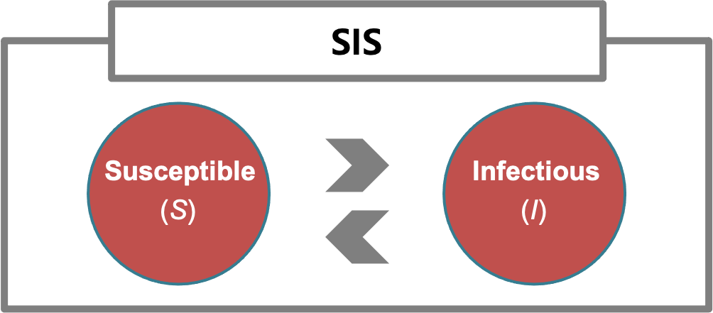
Figure 8.1: A simple SIS model.

Figure 8.2: An SIR model.

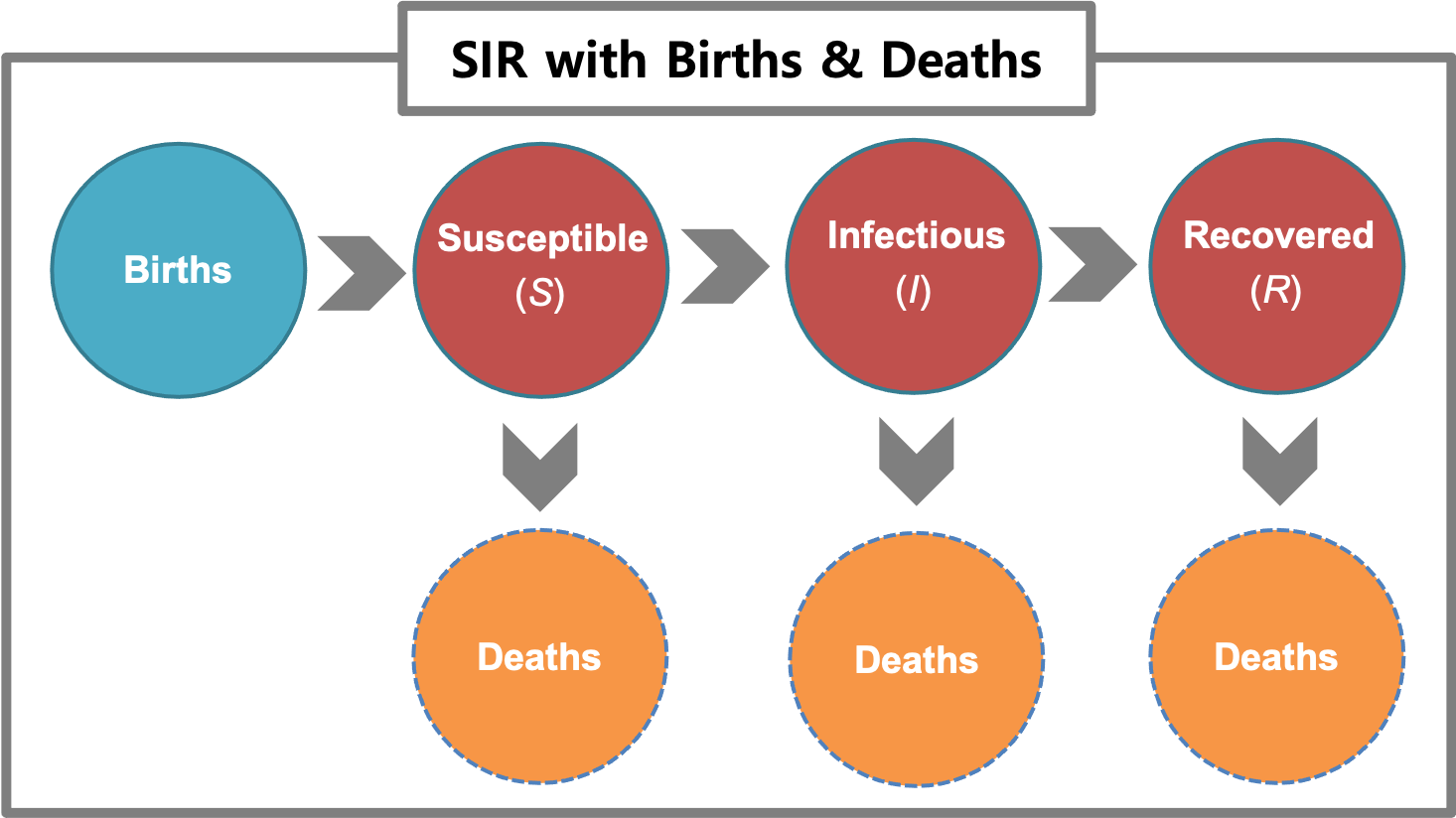
Figure 8.3: An SIR model with birth and death.

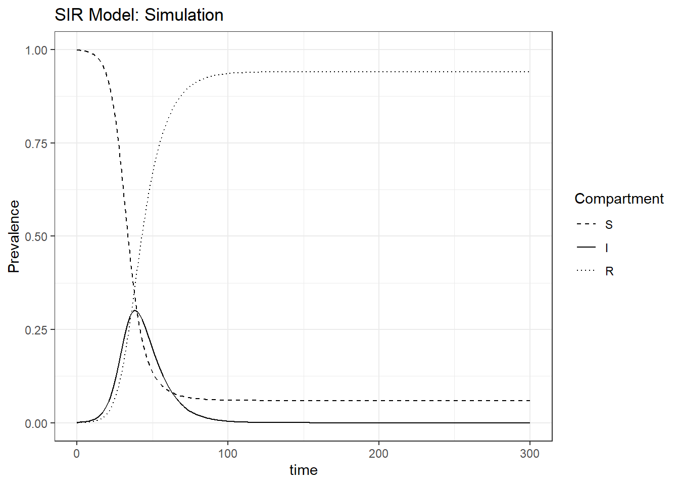
Figure 8.4: Simulation example for compartment model. Top left: prevalence of compartments in the SIR model.

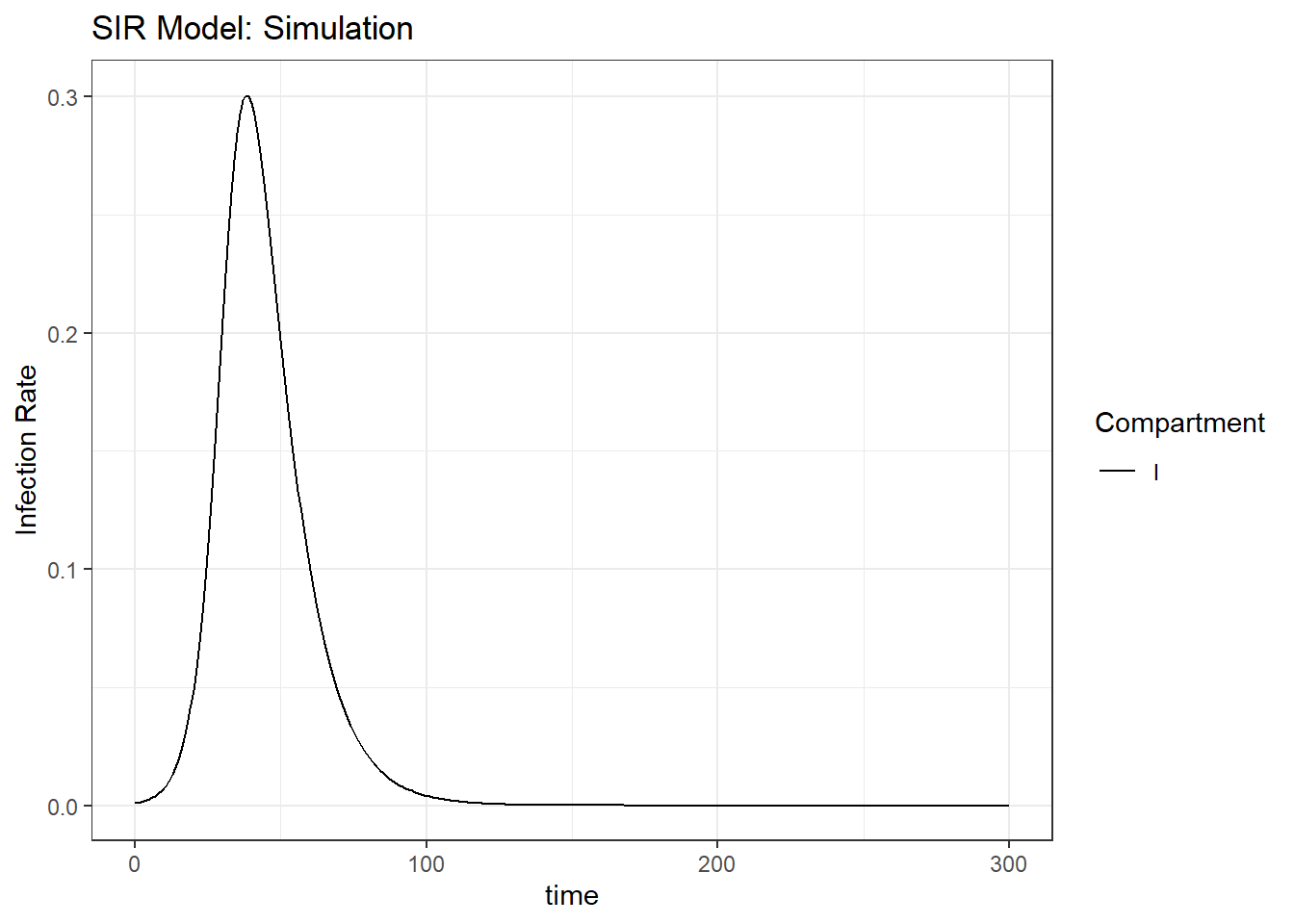
Figure 8.5: Top right: infection rate in the SIR model.

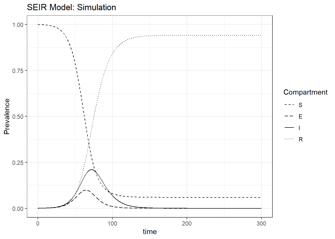
Figure 8.6: Bottom left: prevalence of the SEIR model.

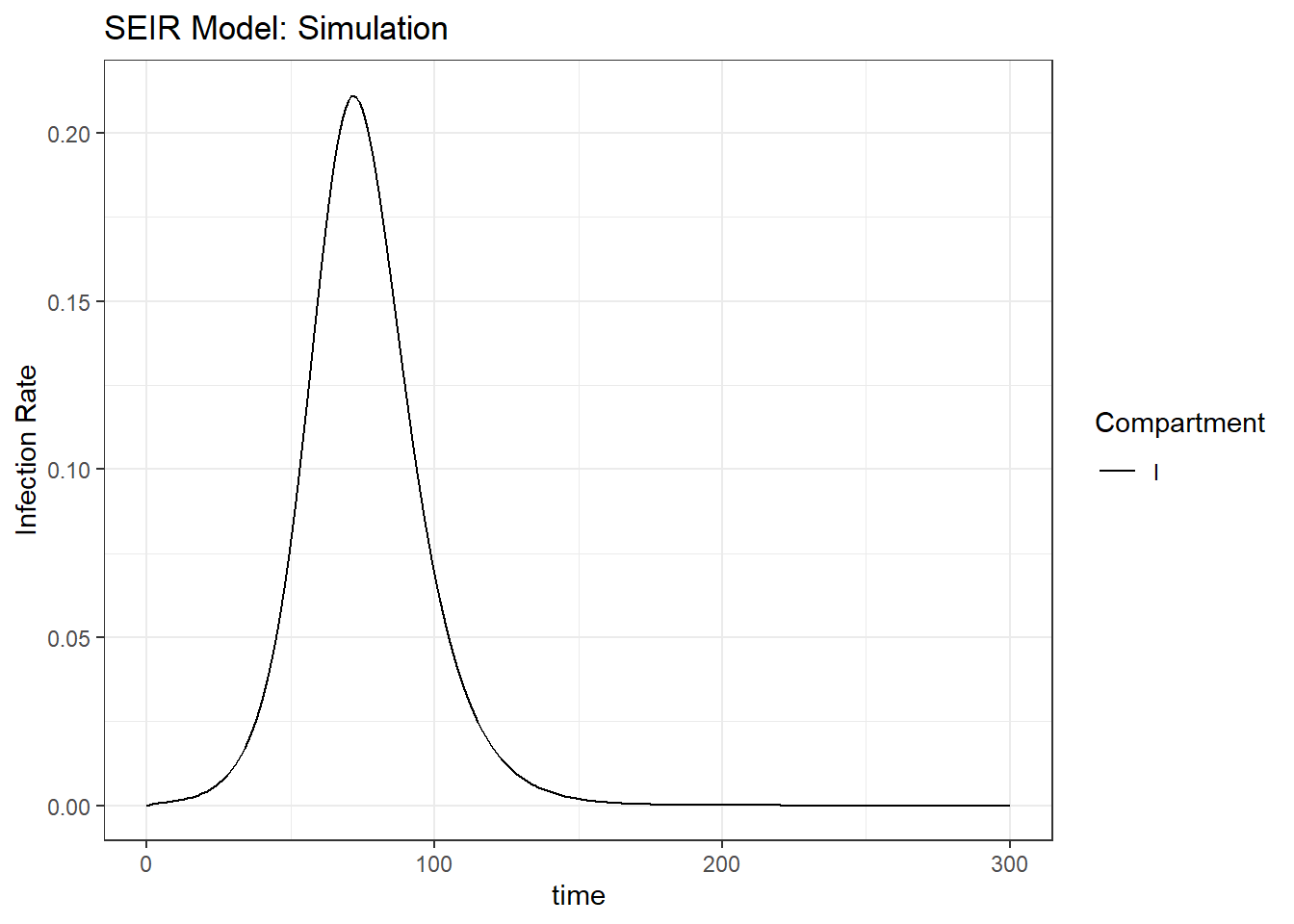
Figure 8.7: Bottom right: infection rate in the SEIR model.

Figure 8.8: The number of patient suffering from ILI for Mid-Atlantic, New England, and Pacific regions from weeks 1 to 24 for the CDC flu season 2016.

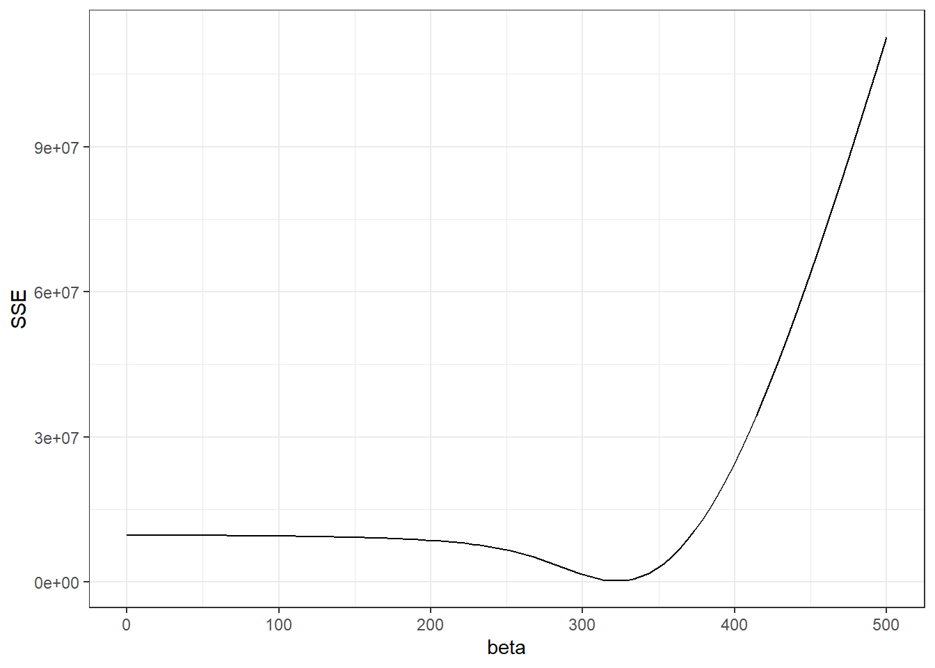
Figure 8.9: Left: SSE values versus \(\beta\) for the least square method.

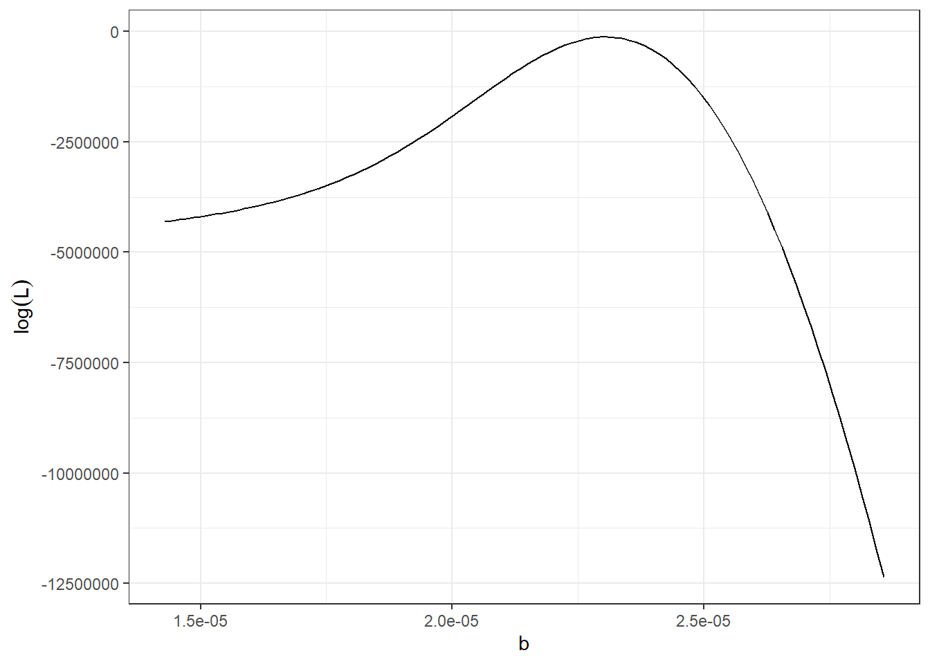
Figure 8.10: Right: log-likelihood function versus \(b\) for the maximum likelihood method.

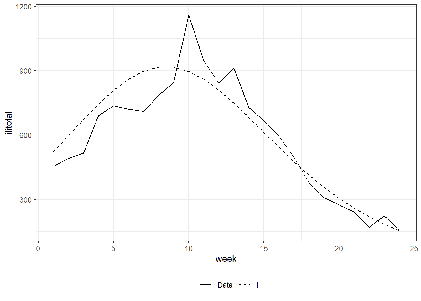
Figure 8.11: The observed path and the fitted curve for \(I(t)\) for the SIR model. Left: least squares method using on grid-searching approach.

Figure 8.12: Middle: least squares method using on general-purpose optimization.

Figure 8.13: Right: maximum likelihood method.

Figure 8.14: The observed path, the fitted and predicted curve for \(I(t)\) based on the lease squares method using general-purpose optimization for the SIR model in the example of COVID-19.

plot(res_parametric_si, legend = FALSE)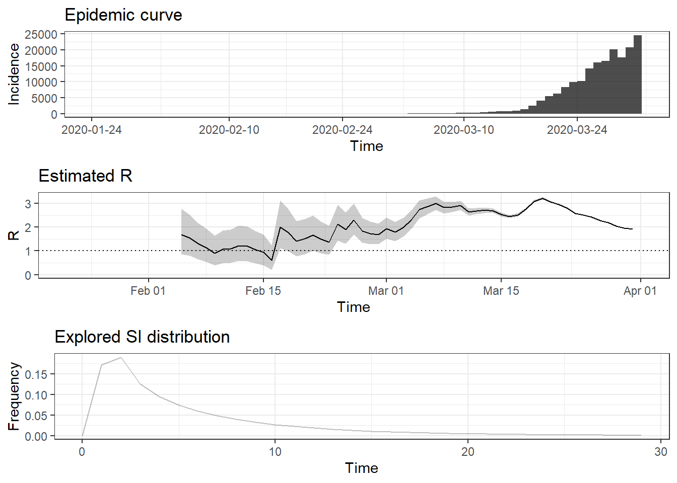

Figure 8.15: Top: time series of incidence. Middle: the estimated effective reproduction number (posterior mean) and 95% credible interval based on parametric_si method and 14-day windows. Bottom: the discrete gamma distribution of the serial interval with the mean 5.52 and sd 5.44, respectively.

plot(res_uncertain_si, legend = FALSE)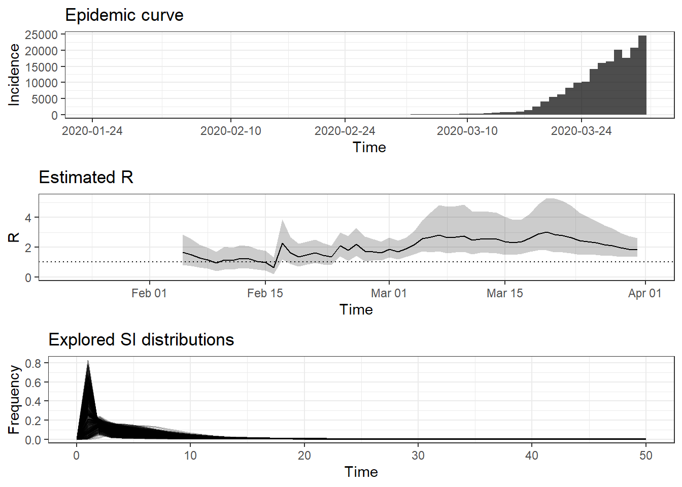

Figure 8.16: Top: time series of incidence. Middle: the estimated effective reproduction number (posterior mean) and 95% credible interval based on uncertain_si method and 14-day windows. Bottom: all the serial interval distributions with the mean and sd sampled from truncated normal distributions with specified parameters.